Embedded zooms
Overview
AGRIF (Adaptive Grid Refinement In Fortran) is a library that allows the seamless space and time refinement over rectangular regions in NEMO. Refinement factors can be odd or even (usually lower than 5 to maintain stability). Interaction between grids is “two-way” in the sense that the parent grid feeds the child grid open boundaries and the child grid provides volume/area weighted averages of prognostic variables once a given number of time steps are completed. This page provide guidelines for how to use AGRIF in NEMO. For a more technical description of the library itself, please refer to AGRIF.
Compilation
Activating AGRIF requires one to add the NST subcomponent and to append the cpp key key_agrif at
compilation time:
./makenemo [...] -d 'OCE ... NST' add_key 'key_agrif'
Although this is transparent to users, the way the code is processed during
compilation is different from the standard NEMO case: a preprocessing stage (the so
called conv program) translates the actual code such that saved arrays may
be switched in memory space from one domain to another.
To avoid compilation issues, it is recommended that you run
./makenemo clean on your configuration the first time you activate
key_agrif if you have previously compiled the configuration.
Definition of the grid hierarchy
Setting up the nested grid location
An additional text file AGRIF_FixedGrids.in is required at run time.
This is where the grid hierarchy is defined. An example of such a file,
taken from the VORTEX test case, is given below:
1
22 41 22 41 3 3 3
0
The first line indicates the number of zooms (1). The second line contains the
start and end indices in both directions on the parent grid
(imin=22 imax=41 jmin=22 jmax=41) followed by the space and time refinement
factors (rx=3 ry=3 rt=3). Each spatial and refinement factor can be chosen
independently (hence one can have a spatial refinement of 3 and a temporal
refinement of 2 for example, even though cfl constraints generally require
these to be the same). The last line is the number of child grids nested in the
refined region, i.e. 0 in this particular case.
The user can find a more complex example in the AGRIF_DEMO reference
configuration directory.
How do I retrieve the exact zoom positioning over the parent grid?
The first/last parent tracer cells inside the zoom (at “T-points” in a C-grid context) will be replaced by volume weighted averages of the child grid values and are given by the following formulae:
Along the i-dimension:
ist = imin + nbghost_w
iend = imax + nbghost_w - 1
Similarly, in the j-dimension:
jst = jmin + nbghost_s
jend = jmax + nbghost_s - 1
The above formulae makes use of nbghost_w and nbghost_s, the number of
ghost cells along the western/southern boundaries, which depends on the
boundary type. The locations of the edges of the zoom, as defined by
imin, imax, etc..., are set excluding the parent ghost cells. The figure
below displays (in the i-dimension) the positioning of two telescoping grids
in a closed domain.
Closed domains have nghost_w = 1 and nghost_s = 1 (there are lines/rows
of masked points on closed domain edges). Global grids will have
nghost_w = 0 and nghost_s = 1 (the western boundary is cyclic, the
southern boundary over Antarctica is closed). AGRIF grids have, by default,
nghost_w = nbghost_s = 4 (as shown in the figure above). One of these ghost
points is masked as required in NEMO. This number, which is not a user defined
parameter, comes from the maximum order of the spatial schemes in the code. A
4th order scheme requires at least 2 unmasked ghost points per time step.
Prather advection as used in the sea-ice model requires 3 ghosts points, which
explains the chosen value.
Hint
It is possible to set a zoom exactly on the edge of a closed parent domain.
Just set imin = 1 to set it on the western edge and/or imax = Ni0glo - 1
to set it on the eastern edge. Same convention in the j dimension.
Dealing with periodic boundaries
If a parent grid has cyclic east-west boundaries or a North-Fold, it is possible to define zooms across the i or j boundaries (as shown in the figure below):
Crossing an east-west boundary requires setting imin < 0, while crossing the
North-Fold needs jmax > Nj0glo.
Hint
It is possible to have a cyclic east-west zoom (e.g. a circumpolar grid),
by setting imin = 1 and imax = Ni0glo+1.
Note
Only a T-point pivot (l_NFold = .T. and c_NFtype = “T”) is currently
supported by AGRIF if one aims at setting a zoom crossing the North-Fold.
Overlapping grids
Rectangular regions must be defined so that they are connected to a single
parent grid. Let’s take as an example the following AGRIF_FixedGrids.in in
the VORTEX test case:
2
22 41 22 41 3 3 3
14 33  8 27 3 3 3
0
0
This will technically “work” as shown by the animation and the code does not complain about such a situation. Nevertheless, this should be avoided because, in the current implementation, grids only exchange data with their parent and not between themselves.
Nested zoom size
From the above formulae, one can get the nested grid size according to:
Ni0glo = (imax-imin)*rx + nbghost_w + nbghost_e
Nj0glo = (jmax-jmin)*ry + nbghost_s + nbghost_n
where the number of ghost cells refer to the child grid (i.e.
nbghost_w=nbghost_e=nbghost_s=nbghost_n=4 in the standard case).
Mesh preprocessing
Once the AGRIF_FixedGrids.in is ready, one has to create a consistent
set of meshes for the whole nested system. This step ensures that cell volumes
agree at the grid interfaces. Volume matching, as well as child bathymetry
interpolation from an external database is ensured by the DOMAINcfg tool
located in /tools/DOMAINcfg/.
Compilation
To compile the DOMAINcfg tool for AGRIF zooms, you need to add
key_agrif (to do so, edit the /tools/DOMAINcfg/cpp_DOMAINcfg.fcm file).
Then, compile:
./maketools [...] -n DOMAINcfg
Creating child meshes
Copy your AGRIF_FixedGrids.in file in your run directory, duplicate
pairs of *_namelist_cfg/ *_namelist_ref files for each grid
and edit them with the expected domain sizes. Alternatively, a python script
can be used to automatically fill child namelists with the expected sizes from
the AGRIF_FixedGrids.in file:
./make_namelist.py namelist_cfg
Specific to the use of AGRIF, two additional namelist options are available for
setting your child grid bathymetry, e.g. through the nn_bathy parameter:
nn_bathy    =    1      ! = 0 compute analyticaly
                        ! = 1 read the bathymetry file
                        ! = 2 compute from external bathymetry
                        ! = 3 compute from parent
Setting nn_bathy=2 creates a child bathymetry from an external bathymetry
database. The database must be stored as a regular (longitude, latitude) array
with the following information required:
cn_topo = 'GEBCO_2020.nc'
cn_bath = 'elevation'
cn_lon = 'lon'
cn_lat = 'lat'
rn_scale = -1
rn_scale=+-1 is a multiplicative factor for negative (rn_scale=-1) or
positive (rn_scale=1) bathymetry values in input file. Interpolation is
performed using a median average and a “lake-filling” algorithm removes
any small wet domains not connected to the zoom edges. One can simply use the
parent bathymetry as the bathymetry source by setting nn_bathy=3. One can
still read a bathymetry file over the child domain by setting nn_bathy=1
as long as it exactly corresponds to the expected domain size and position.
This can be used to re-run the tool after hand editing the coastline for example.
Hint
At this stage, you can change the vertical grid definition in
each zoom (only ln_zps grid types are fully functional though) which
requires setting ln_vert_remap=T in the namagrif namelist block.
This also requires setting ln_dept_mid=T in ALL namelists, vertical
remapping being only compatible with a mid-cell location of T-points.
Then, run the executable (eventually on multiple cores):
mpirun -np [...] ./make_domain_cfg.exe
This creates an updated domain_cfg.nc root mesh and all the child meshes
1_domain_cfg.nc, 2_domain_cfg.nc, etc…
Hint
Even with the same vertical grid, a child domain may need fewer vertical
levels than jpkglo. Check your *_ocean.output which gives you the
maximum number of levels required. Adjust the number of levels
(jpkglo only, leaving jpkdta unchanged) in the namelists, and
re-run DOMAINcfg a second time.
You may take as an example the AGRIF_DEMO case located in the
/tool/DOMAINcfg/cfgs/AGRIF_DEMO directory. This particular case
illustrates a vertical coordinate change for the last zoom level.
Running the multigrid system
Input files
Each child grid expects to read its own namelist so that different numerical
choices can be made (these should be stored in the form 1_namelist_cfg,
2_namelist_cfg, etc… according to their rank in the grid hierarchy).
Copy the mesh files obtained in the preprocessing step above in your run directory.
Note that variable names in child namelists should not contain the grid prefixes which
are added at run time. Hence, reading for example the child mesh 1_domain_cfg.nc requires
setting in your namelist:
!-----------------------------------------------------------------------
&namcfg        !   parameters of the configuration
!-----------------------------------------------------------------------
ln_read_cfg = .true.              !  (=T) read the domain configuration file
   cn_domcfg = "domain_cfg.nc"    ! domain configuration filename
/
The same applies to interpolation weights, restarts, runoffs files, etc… if any. Namelists could be at the end pretty much similar for all grids.
Note
The land/sea mask and the vertical grid of the parent grid might have
been modified over the nest(s) area(s) by the DOMAINcfg tool
(because of the volume matching). Therefore, make sure that your input files are consistent.
Note
To ensure that child time parameters agree with the chosen temporal refinement,
nn_it000, nn_itend and rn_Dt (e.g. first and last time steps and the time
step increment in the namelist) are all overwritten at run time according to
the parent values and the time refinement factor rt.
Ouput files
Outputs are produced as for single grid experiments, thanks to the XIOS library.
Definitions in your file_def_nemo-XXX.xml file will lead to a set of Netcdf files but
with the grid prefix. The only change required by the user is the addition of a
context_nemo.xml file for each grid in iodef.xml:
 <!-- ============================================================================================ -->
 <!-- NEMO  CONTEXT add and suppress the components you need                                       -->
 <!-- ============================================================================================ -->

<context id="nemo" src="./context_nemo.xml"/>       <!--  ROOT       -->e
<context id="1_nemo" src="./1_context_nemo.xml"/>   <!--  GRD1       -->
<context id="2_nemo" src="./2_context_nemo.xml"/>   <!--  GRD2       -->
</simulation>
Then, duplicate context_nemo.xml files accordingly and edit the id name 1_nemo,
etc… in each of them.
Hint
It is possible to output different variables on each grid. Simply copy file_def_nemo-XXX.xml
as 1_file_def_nemo-XXX.xml for example and change the file name in 1_context_nemo.xml.
Namelist options specific to AGRIF
Specific to AGRIF is the following namelist block:
!-----------------------------------------------------------------------
&namagrif      !  AGRIF zoom                                            ("key_agrif")
!-----------------------------------------------------------------------
ln_agrif_2way   = .true.  !  activate two way nesting
ln_init_chfrpar = .false. !  initialize child grids from parent
ln_vert_remap   = .false. !  use vertical remapping
ln_spc_dyn      = .false. !  use 0 as special value for dynamics
ln_chk_bathy    = .true.  !  =T  check the parent bathymetry
rn_sponge_tra   = 0.002   !  coefficient for tracer   sponge layer []
rn_sponge_dyn   = 0.002   !  coefficient for dynamics sponge layer []
rn_trelax_tra   = 0.01    !  inverse of relaxation time (in steps) for tracers []
rn_trelax_dyn   = 0.01    !  inverse of relaxation time (in steps) for dynamics []
/
!-----------------------------------------------------------------------
Sponge/relaxation parameters (rn_sponge_xxx/rn_trelax_xxx) control the possible noise
near grid interfaces. These are non-dimensionalized parameters and do not require, in principle, to be
systematically adjusted to your setup.
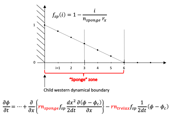
The following figure describes, here in one dimension, the location of the zone
near a western child boundary and the linear decrease of the sponge/relaxation coefficient. Note that the width of the zone, in number of parent (coarse) grid points, is a parameter defined in the code (nsponge = 2 by default). The equation displays the aditionnal terms involved and where the namelist parameters intervene.
A last useful option is ln_init_chfrpar=T which skips any external
initialization for the child grid by setting the initial state from its parent
level.
Note
the ln_vert_remap flag must be activated if different vertical
grids are used in the parent and the child grids.
Unsupported options with AGRIF
A number of features are not compatible with the key_agrif defined. In most of
the cases listed below it simply means that the functionality has not been adapted to the
multigrid paradigm. For example, activating icebergs would ideally require Lagrangian
parcels being able to transit from one grid to another, which has not been implemented.
The missing functionalities are grouped in the table below according to their use on the
root or on the child grid.
Option name (and flag) |
Grid |
|
|---|---|---|
Root |
Child |
|
Timing ( |
No |
|
Icebergs ( |
No |
|
Under ice shelves cavities ( |
No |
No |
Floats ( |
No |
|
Stochastic param. ( |
No |
|
Open boundaries ( |
Yes |
No |
Global heat and salt budgets ( |
No |
|