Migrating from 4.0.x to 4.2.x

Modification of input and output files

Up to NEMO version 4.0.x (inclusive), if the domain configuration includes one of the possible periodicity conditions (East-West (EW), North-South (SN) or North-Pole (NP) folding), all input and output files include extra columns and/or rows used to implement the periodicity, see Figure 1.:

In EW periodicity, the first and last columns are duplicated.

In the SN periodicity, the first and last rows are duplicated.

The NP folding requires the duplication of (at least) the last row.

Note that, NP folding also includes the EW periodicity (jperio = 1).

The bi-periodicity (jperio = 7) is the combination of jperio = 1 and 2.

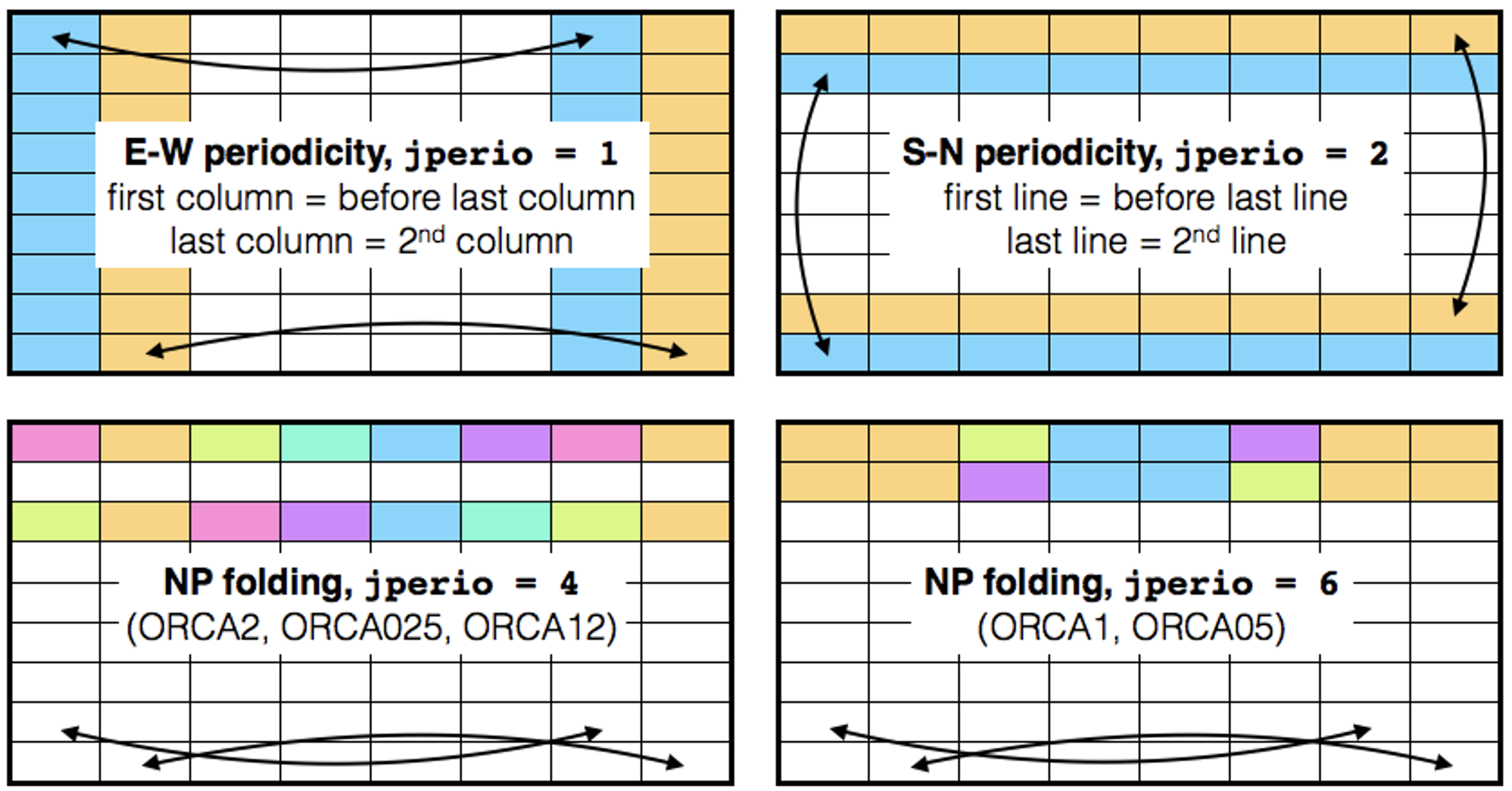
Figure 1: Columns and/or rows duplication included in input/output files according to the chosen periodicity. Thick black rows delimit the part of the domain included in all input/outputs files.

From NEMO 4.2.0, the columns and rows that are duplicated because of periodicity (EW, SN and NP) are excluded from all input and output files. In practice, when preparing old configurations for use with 4.2.0, this means:

In EW periodicity, the first and last columns are removed.

For the SN periodicity, the top and bottom rows are removed

The last row is also removed when using the NP folding

Closed boundary conditions are unchanged and still require a

column or a row of land points

These changes are illustrated in Figure 2.

If we consider for example the ORCA2 grid, up to version 4.0.x (included), the grid size is (182/149). From version 4.2.0, its size becomes (180/148) as the first and last columns have been removed because of the EW periodicity, and as the last row has been removed because of the NP folding. The southern boundary is untouched as it is closed by a row of land points.

Note that, in NP folding case, there is often more than the last row, which is duplicated. For NP fording around the “T” point, 1.5(2) rows are replicated for the grids T and U (V and F). The folding around the “F” point requires duplication of 1(1.5) rows for grids T and U (V and F). We however decided to remove only the last row in all cases to make things simpler. In consequence, even with the top row removed, the input and output files may still contain duplicated points depending of the grid type and the NP folding case.

The simplest way to use the input files for version <= 4.0.x with version >= 4.2.0 is to cut the extra columns and rows in the input files with a command like ncks -F -d or cdo selindexbox. Note that the sides of the domain which correspond to closed boundaries must not been changed for the revision 4.2.0. Here is and example on how to rewrite the domcfg file of ORCA2 from 4.0.x to 4.2.0:

ncks -F -d x,2,181 -d y,1,148 ORCA2_r4.0.x_domcfg.nc ORCA2_r4.2.0_domcfg.nc

This simple cut of the columns and rows can also be applied to the weights files used for the on-the-fly interpolation.

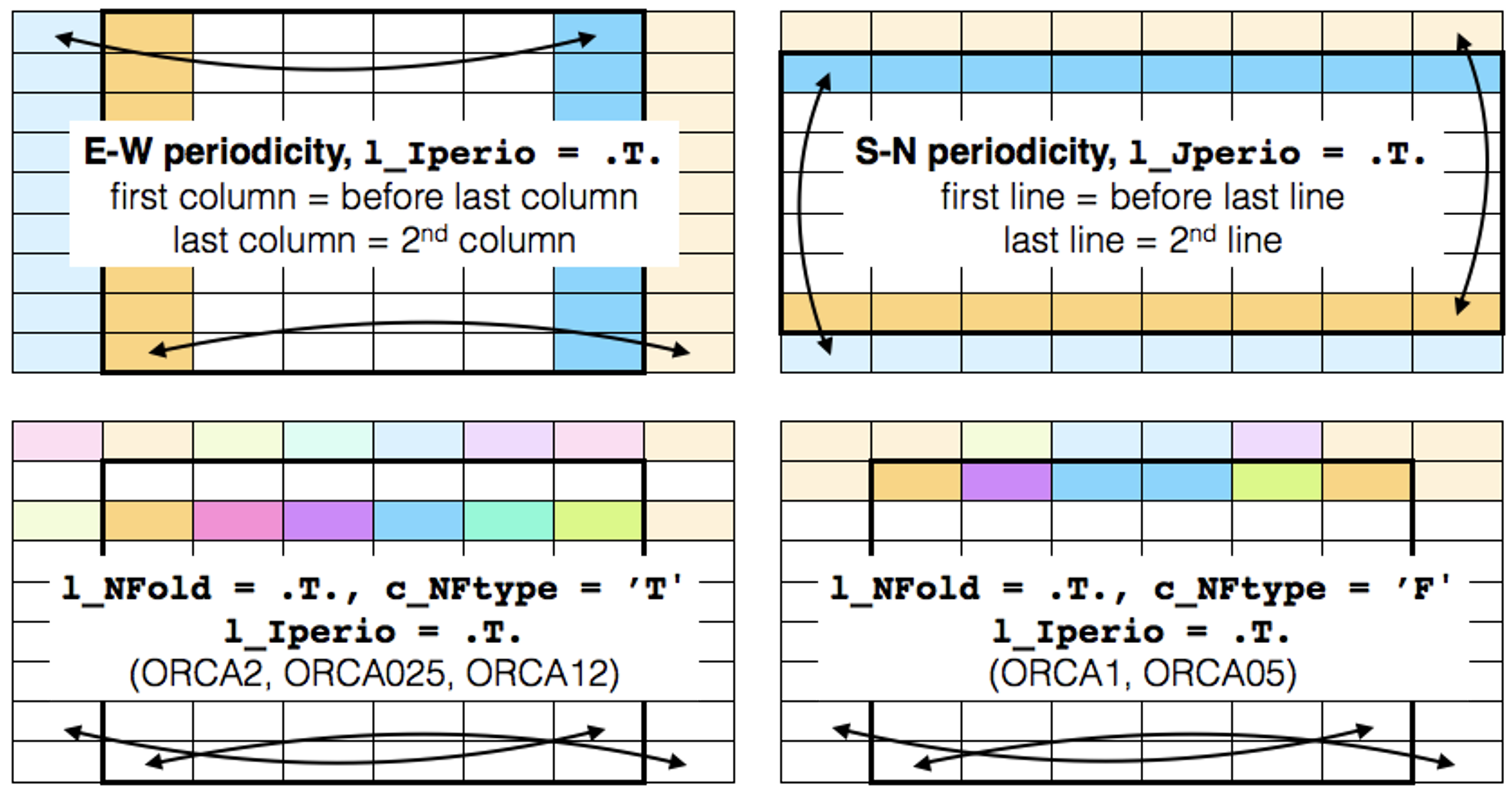
Figure 2: Exclusion of the duplicated columns and rows according to the chosen periodicity. Thick black rows delimit the part of the domain included in all input/outputs files. Light colour cells are no longer required.

Even when extra columns and rows used for periodicity (light colours in Figure 2) are excluded from the input and output files, they are still needed during the code integration. They are therefore recreated during code execution and the grid size in the input and output files is thus different from the grid size inside the code. The values of the additional columns and/or rows are automatically defined at run-time by applying the proper boundaries conditions (by means of a call to the lbc_lnk routine).

From 4.2.0, the grid size inside the code depends on the number of MPI halos (nn_hls in the namelist). We add nn_hls columns/rows in each direction, even if the boundary is closed. This last point differs from what was done before the version 4.2.0. If the domain contains one or more closed boundaries, its domain size inside the code will differ before and after the version 4.2.0, even if nn_hls = 1. For example, with ORCA2, the grid size inside the code was (182/149), it will be, from the 4.2.0, (182/150) if nn_hls = 1 or (184/152) if nn_hls = 2. Note that, as the MPI domain decomposition depends of the grid size inside the code, it will therefore change according to the value of nn_hls. If the domain contains a closed boundary, the MPI domain decomposition won’t be the same before and after the version 4.2.0, even if nn_hls = 1 and even if we fix the number of MPI of subdomains in the i and j directions (with jpni and jpnj in the namelist).

The way we define the type of periodicity has also been reviewed from version 4.2.0. We replaced jperio by several, more explicit variables. The table bellow details the equivalent of the different values of jperio from revision 4.2.0.

<= 4.0.x	>= 4.2.0
jperio = 0	l_Iperio = .F., l_Jperio = .F., l_NFold = .F.
jperio = 1	l_Iperio = .T., l_Jperio = .F., l_NFold = .F.
jperio = 2	l_Iperio = .F., l_Jperio = .T., l_NFold = .F.
jperio = 3	l_Iperio = .F., l_Jperio = .F., l_NFold = .T., c_NFtype = “T”
jperio = 4	l_Iperio = .T., l_Jperio = .F., l_NFold = .T., c_NFtype = “T”
jperio = 5	l_Iperio = .F., l_Jperio = .F., l_NFold = .T., c_NFtype = “F”
jperio = 6	l_Iperio = .T., l_Jperio = .F., l_NFold = .T., c_NFtype = “F”
jperio = 7	l_Iperio = .T., l_Jperio = .T., l_NFold = .F.

Following these modifications we also changed the way options are defined in domcfg files. All options are now defined with NetCDF global attributes instead of scalar variables. This is more readable and easier to manipulate with commands like ncatted. The following table details which attributes replace which scalar variable. Note that the 4.2.0 code is still able to read the old domcfg files with the options defined with scalar variables (including the automatic translation from jperio to the new varaibles listed in the above table).

<= 4.0.x	>= 4.2.0
NetCDF scalar variables	NetCDF global attributes
jpiglo	Automatically defined with the 1st dimension of the variable e3t_0
jpjglo	Automatically defined with the 2nd dimension of the variable e3t_0
jpkglo	Automatically defined with the 3rd dimension of the variable e3t_0
jperio	Iperio = 0 or 1, 0 by default Jperio = 0 or 1, 0 by default NFold = 0 or 1, 0 by default NFtype = “T”, “F”, “-” by default
ORCA	CfgName = any character string, ‘UNKNOWN’ by default
ORCA_index	CfgIndex = any integer, -999 by default
ln_zco = 1.	VertCoord = “zco”, “-” by default
ln_zps = 1.	VertCoord = “zps”, “-” by default
ln_sco = 1.	VertCoord = “sco”, “-” by default
ln_isfcav	IsfCav = 0 or 1, 0 by default

Here is an example on how to create global attributes with the command ncatted:

ncatted -a Iperio,global,c,l,1 -a NFtype,global,c,c,'T' domcfg.nc

Speed up associated with reduced memory requirements

In order to reduce the memory footprint in NEMO 4.2, an additional way of dealing with vertical scale factors has been implemented using cpp keys (key_linssh, key_qco). These keys allow a reduction of the memory footprint by removing 26 x 3D arrays at the cost of 10 x 2D arrays. In tests without I/O, this implementation allows a speed up of 7 to 15% depending on the average memory load among processors.

There are 4 distinct vertical coordinates, namely: fixed coordinates (ln_linssh=T) , variable zstar coordinates (ln_linssh=F & ln_vvl_zstar=T) , variable ztilde coordinates (ln_linssh=F & ln_vvl_tilde=T) and variable zlayer coordinates (ln_linssh=F & ln_vvl_layer=T ). The optimization has only been implemented for fixed and zstar vertical coordinates but it will be generalized to all coordinates in future releases. Users are encouraged to use it for their applications.

<= 4.0.x	>= 4.2.0
ln_linssh=T	ln_linssh=T & compile with key_linssh
ln_linssh=F , ln_vvl_zstar=T	ln_linssh=F , ln_vvl_zstar=T & compile with key_qco
ln_linssh=F , ln_vvl_zlayer=T	ln_linssh=F , ln_vvl_zlayer=T
ln_linssh=F , ln_vvl_ztilde=T	ln_linssh=F , ln_vvl_ztilde=T

Note

In the cases when you use key_linssh or key_qco you must also set the namelist parameter ln_linssh accordingly.

In the case of fixed vertical scale factors, in addition to setting the namelist parameter ln_linssh = .true., compiling the code with key_linssh is recommended. The use of the key avoids the duplication of variables such as scale factors and water depth. Instead it substitutes them with time invariant arrays. For instance:

#   define  gdept(i,j,k,t) gdept_0(i,j,k)

In the case of varying vertical scale factors with zstar coordinates, in addition to setting the namelist parameter ln_linssh = .false., compile the code with key_qco. QCO stands for Quasi-eulerian COordinates and it replaces VVL (Vertical Varying Layer). In practice, each vertical level varies linearly with respect to ssh. Therefore, time evolution of the vertical scale factors can be expressed as a function of ssh to h ratio (r3 = ssh/h) and 4D arrays can be substituted by simple expressions. For instance:

#   define  e3t(i,j,k,t)   (e3t_0(i,j,k)*(1._wp+r3t(i,j,t)*tmask(i,j,k)))

For ice-shelf simulations, a key_isf cpp key is needed in addition to key_qco, so that water depth expressions gdept and gdepw take the ice-shelf depth into account:

#   define  gdept(i,j,k,t) ((gdept_0(i,j,k)-risfdep(i,j))*(1._wp+r3t(i,j,t))+risfdep(i,j))

In the case of varying vertical scale factors with other coordinates, do not apply the key_linssh or key_qco keys.

Note

This optimisation is currently not working with ztilde nor layer options for vertical scale factors.

Shallow Water

The SWE (Shallow Water Equation) module (./src/SWE) is a demonstrator for shallow water equations newly included in NEMO v4.2. This module is an early demonstrator for the changes to the time-stepping scheme that are planned for the next release. It contains suitable shallow water time stepping routines for both Modified Leap Frog (stpmlf.F90) and Runge Kutta 3rd order (stprk3.F90) time schemes. Note that in the MLF case, the key_qco compilation pre-processing key is needed. RK3 requires both key_qco and either key_RK3 or key_RK3all compilation pre-processing keys. RK3 time-stepping is a 3 stage algorithm: 1st and 2nd stages build estimates of intermediate fields, the 3rd stage integrates the model from n to n+1 using the intermediate estimates. With key_RK3all, all the stages are integrated with the full suite of ocean dynamics including advection, vorticity, lateral diffusion, pressure gradient, and forcing. Instead, with key_RK3, lateral diffusion and forcing are removed from stages 1 and 2.