Run the Reference configurations

Note

Lack of illustrations for ref. cfgs, and more generally in the guide.

NEMO is distributed with a set of reference configurations allowing both the user to set up his own first applications and the developer to test/validate his NEMO developments (using SETTE package).

Attention

Concerning the configurations, the NEMO System Team is only in charge of the “Reference Configurations” described below.

Hint

Configurations developed by external research projects or initiatives that make use of NEMO are welcome to be publicized through the website by filling up the form Add your project here and Add your publications here

How to compile an experiment from a reference configuration

To compile the ORCA2_ICE_PISCES reference configuration using makenemo, one should use the following, by selecting among available architecture file or providing a user defined one:

$ ./makenemo -r 'ORCA2_ICE_PISCES' -m 'my_arch' -j '4'

A new EXP00 folder will be created within the selected reference configurations, namely ./cfgs/ORCA2_ICE_PISCES/EXP00. It will be necessary to uncompress the archives listed in the above table for the given reference configuration that includes input & forcing files.

Then it will be possible to launch the execution of the model through a runscript (opportunely adapted to the user system).

List and description of Reference Configurations

All forcing files listed below in the table are available from the SETTE inputs site . Note, this list also includes two configurations in the test-cases category. These latter two are located in the tests directory

Configuration	Component(s)					Archives (input & forcing files)
Name	O	S	T	P	A
AGRIF_DEMO	X	X	X		X	AGRIF_DEMO_v4.2.0.tar, ORCA2_ICE_v4.2.0.tar
AMM12	X					AMM12_v4.2.0.tar
C1D_PAPA	X					C1D_PAPA_v4.2.0.tar
GYRE_PISCES	X		X	X		none
ORCA2_ICE_PISCES	X	X	X	X		ORCA2_ICE_v4.2.0.tar
ORCA2_OFF_PISCES			X	X		ORCA2_OFF_v4.2.0.tar
ORCA2_OFF_TRC			X			ORCA2_OFF_v4.2.0.tar
ORCA2_SAS_ICE		X				ORCA2_ICE_v4.2.0.tar, SAS_v4.2.0.tar
WED025	X	X				WED025_v4.2.0.tar
ICE_AGRIF	X	X			X	ICE_AGRIF.2.0.tar
ISOMIP+_	X					ISOMIP+_4.2.0.tar

Legend for component combination

O for OCE, S for SI³, T for TOP, P for PISCES and A for AGRIF

AGRIF_DEMO

AGRIF_DEMO is based on the ORCA2_ICE_PISCES global configuration at 2° of resolution with the inclusion of 3 online nested grids to demonstrate the overall capabilities of AGRIF in a realistic context (including the nesting of sea ice models).

The configuration includes a 1:1 grid in the Pacific and two successively nested grids with odd and even refinement ratios over the Arctic ocean, with the finest grid (1/6°) spanning the Denmark strait that is of particular interest to test sea ice coupling. Noteworthy, this last zoom benefits from the “vertical nesting” capacity introduced in v4.2. It has a 75 levels geopotential grid (which is not an integer refinement of the 30 levels parent grid), while still allowing for conservative 2-way exchanges. To test passive tracer exchanges through AGRIF, an Age tracer is also activated.

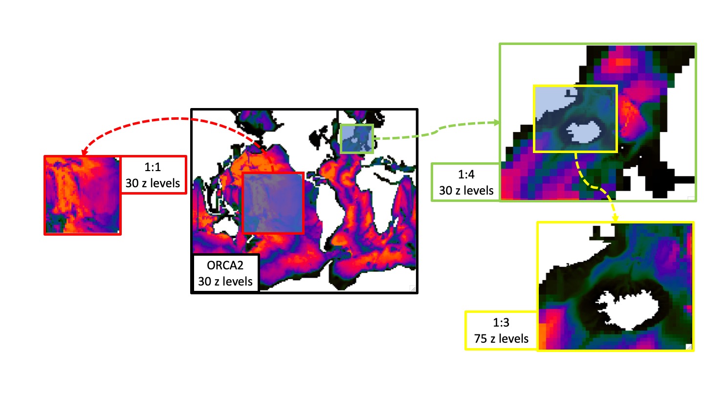
The 1:1 grid can be used alone as a benchmark to check that the model solution is not corrupted by grid exchanges. Note that since grids interact only at the baroclinic time level, numerically exact results can not be achieved in the 1:1 case. Perfect reproducibility is obtained only by switching to a fully explicit setup instead of a split explicit free surface scheme.

AMM12

AMM12 stands for Atlantic Margin Model at 12 km that is a regional configuration covering the Northwest European Shelf domain on a regular horizontal grid of ~12 km of resolution (see [C1]).

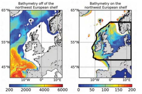
This configuration allows to tests several features of NEMO specifically addressed to the shelf seas. In particular, AMM12 accounts for vertical s-coordinates system, GLS turbulence scheme, tidal lateral boundary conditions using a flather scheme (see more in BDY). Boundaries may be completely omitted by setting ln_bdy = .false. in nambdy.

Sample surface fluxes, river forcing and an initial restart file are included to test a realistic model run (AMM12_v4.2.0.tar).

Note that, the Baltic boundary is included within the river input file and is specified as a river source, but unlike ordinary river points the Baltic inputs also include salinity and temperature data.

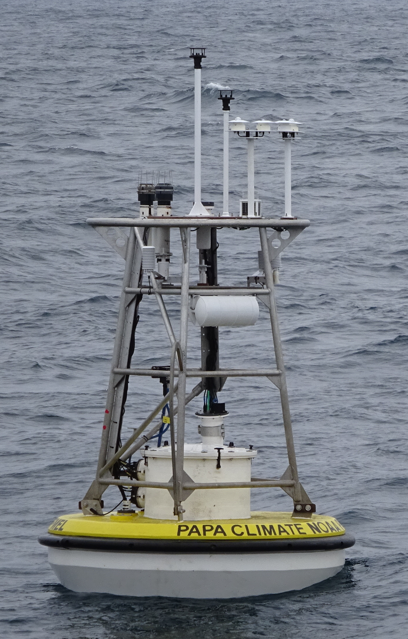
C1D_PAPA

C1D_PAPA is a 1D configuration for the PAPA station located in the northern-eastern Pacific Ocean at 50.1°N, 144.9°W. See Reffray et al. (2015) for the description of its physical and numerical turbulent-mixing behaviour.

The water column setup, called NEMO1D, is activated by setting ln_c1d = .true. in namdom and has a horizontal domain of 1x1 grid point.

This reference configuration uses 75 vertical levels grid (1m at the surface), GLS turbulence scheme with K-epsilon closure and the NCAR bulk formulae.

Data provided with INPUTS_C1D_PAPA_v4.2.0.tar file account for:

Input files in C1D_v4.2.0.tar: forcing_PAPASTATION_1h_y201[0-1].nc:

ECMWF operational analysis atmospheric forcing rescaled to 1h (with long and short waves flux correction) for years 2010 and 2011, init_PAPASTATION_m06d15.nc: Initial Conditions from observed data and Levitus 2009 climatology,and chlorophyll_PAPASTATION.nc: surface chlorophyll file from Seawifs data

GYRE_PISCES

GYRE_PISCES is an idealized configuration representing a Northern hemisphere double gyres system, in the Beta-plane approximation with a regular 1° horizontal resolution and 31 vertical levels, with PISCES BGC model [C2]. Analytical forcing for heat, freshwater and wind-stress fields are applied.

This configuration acts also as demonstrator of the user defined setup (ln_read_cfg = .false.) and grid setting are handled through the &namusr_def controls in namelist.cfg, lines 35-41 :

Note that, the default grid size is 30x20 grid points (with nn_GYRE = 1) and vertical levels are set by jpkglo. The specific code changes can be inspected in ./src/OCE/USR.

Running GYRE as a benchmark

This simple configuration can be used as a benchmark since it is easy to increase resolution, with the drawback of getting results that have a very limited physical meaning.

GYRE grid resolution can be increased at runtime by setting a different value of nn_GYRE (integer multiplier scaling factor), as described in the following table:

nn_GYRE	jpiglo	jpjglo	jpkglo	Equivalent to
1	30	20	31	GYRE 1°
25	750	500	101	ORCA 1/2°
50	1500	1000	101	ORCA 1/4°
150	4500	3000	101	ORCA 1/12°
200	6000	4000	101	ORCA 1/16°

Note that, it is necessary to set ln_bench = .true. in &namusr_def to avoid problems in the physics computation and that the model timestep should be adequately rescaled.

For example if nn_GYRE = 150, equivalent to an ORCA 1/12° grid, the timestep rn_rdt should be set to 1200 seconds Differently from previous versions of NEMO, the code uses by default the time-splitting scheme and internally computes the number of sub-steps.

ORCA2_ICE_PISCES

ORCA2_ICE_PISCES is a reference configuration for the global ocean with a 2°x2° curvilinear horizontal mesh and 31 vertical levels, distributed using z-coordinate system and with 10 levels in the top 100m. ORCA is the generic name given to global ocean Mercator mesh, (i.e. variation of meridian scale factor as cosinus of the latitude), with two poles in the northern hemisphere so that the ratio of anisotropy is nearly one everywhere

This configuration uses the three components

• NEMO-OCE, the ocean dynamical core

• NEMO-SI³, the thermodynamic-dynamic sea ice model.

• NEMO-TOP, passive tracer transport module and PISCES BGC model [C2]

All components share the same grid. The model is forced with CORE-II normal year atmospheric forcing and it uses the NCAR bulk formulae.

Ocean Physics

horizontal diffusion on momentum

the eddy viscosity coefficient depends on the geographical position. It is taken as 40000 m²/s, reduced in the equator regions (2000 m²/s) excepted near the western boundaries.

isopycnal diffusion on tracers

the diffusion acts along the isopycnal surfaces (neutral surface) with an eddy diffusivity coefficient of 2000 m²/s.

Eddy induced velocity parametrization

With a coefficient that depends on the growth rate of baroclinic instabilities (it usually varies from 15 m²/s to 3000 m²/s).

lateral boundary conditions

Zero fluxes of heat and salt and no-slip conditions are applied through lateral solid boundaries.

bottom boundary condition

Zero fluxes of heat and salt are applied through the ocean bottom. The Beckmann [19XX] simple bottom boundary layer parameterization is applied along continental slopes. A linear friction is applied on momentum.

convection

The vertical eddy viscosity and diffusivity coefficients are increased to 1 m²/s in case of static instability.

time step

is 5400sec (1h30’) so that there is 16 time steps in one day.

ORCA2_OFF_PISCES

ORCA2_OFF_PISCES is based on the ORCA2 global ocean configuration (see ORCA2_ICE_PISCES for general description) along with the tracer passive transport module (TOP), but dynamical fields are pre-calculated and read with specific time frequency.

This enables for an offline coupling of TOP components.

Pre-calculated dynamical fields are provided to NEMO using the namelist &namdta_dyn in namelist_cfg, in this case with a 5 days frequency (120 hours):

Input dynamical fields for this configuration (ORCA2_OFF_v4.2.0.tar) comes from a 2000 years long climatological simulation of ORCA2_ICE using ERA40 atmospheric forcing.

Note that, this configuration default uses linear free surface (ln_linssh = .true.) assuming that model mesh is not varying in time and it includes the bottom boundary layer parameterization (ln_trabbl = .true.) that requires the provision of BBL coefficients through sn_ubl and sn_vbl fields.

It is also possible to activate a user defined set of tracers and source-sink terms with ln_my_trc = .true. (and adaptation of ./src/TOP/MY_TRC routines).

In addition, the offline module (OFF) allows for the provision of further fields:

1. River runoff can be provided to TOP components by setting ln_dynrnf = .true. and by including an input datastream similarly to the following:

   sn_rnf  = 'dyna_grid_T', 120, 'sorunoff' , .true., .true., 'yearly', '', '', ''
   

2. VVL dynamical fields, in the case input data were produced by a dyamical core using variable volume (ln_linssh = .false.) it is necessary to provide also diverce and E-P at before timestep by including input datastreams similarly to the following

   sn_div  = 'dyna_grid_T', 120, 'e3t'      , .true., .true., 'yearly', '', '', ''
   sn_empb = 'dyna_grid_T', 120, 'sowaflupb', .true., .true., 'yearly', '', '', ''
   

More details can be found by inspecting the offline data manager in the routine ./src/OFF/dtadyn.F90.

ORCA2_SAS_ICE

ORCA2_SAS_ICE is a demonstrator of the Stand-Alone Surface (SAS) module and it relies on ORCA2 global ocean configuration (see ORCA2_ICE_PISCES for general description).

The standalone surface module allows surface elements such as sea-ice, iceberg drift, and surface fluxes to be run using prescribed model state fields. It can profitably be used to compare different bulk formulae or adjust the parameters of a given bulk formula.

More informations about SAS can be found in NEMO manual.

WED025

WED025 is a regional configuration of the Weddell sea region at 1/12° of horizontal resolution and 75 vertical levels. See [C3] for more details.

This configuration references to year 2002, with atmospheric forcing provided every 2 hours using NCAR bulk formulae, while lateral boundary conditions for dynamical fields have 3 days time frequency.

References

C1

E. J. O’Dea, A. K. Arnold, K. P. Edwards, R. Furner, P. Hyder, M. J. Martin, J. R. Siddorn, D. Storkey, J. While, J. T. Holt, and H. Liu. An operational ocean forecast system incorporating nemo and sst data assimilation for the tidally driven european north-west shelf. Journal of Operational Oceanography, 5(1):3–17, Feb 2012. doi:10.1080/1755876x.2012.11020128.

C2(1,2)

O. Aumont, C. Ethé, A. Tagliabue, L. Bopp, and M. Gehlen. Pisces-v2: an ocean biogeochemical model for carbon and ecosystem studies. Geoscientific Model Development, 8(8):2465–2513, Aug 2015. doi:10.5194/gmd-8-2465-2015.

C3

C. Rousset, M. Vancoppenolle, G. Madec, T. Fichefet, S. Flavoni, A. Barthélemy, R. Benshila, J. Chanut, C. Levy, S. Masson, and F. Vivier. The louvain-la-neuve sea ice model lim3.6: global and regional capabilities. Geoscientific Model Development, 8(10):2991–3005, 2015. doi:10.5194/gmd-8-2991-2015.